2012-08-03

My First MySQL session


First of all, installing the MySQL Data Base Management System is a straightforward process. I used Synaptic to install the mysql-server and mysql-client packages on my Linux platform. If you use Windows you can visit the download page at mysql.com.


This is an example of a simple MySQL session. The commands are self-explanatory. If you need a little bit more of a walk-through, the "MySQL Tutorial for beginners" series on YouTube is a step-by-step description of most of the commands that follow.
1. Creating a database and adding tables to it   (8:49 min)
2. Adding data to tables in a database   (5:49 min)
3. Selecting data from tables in a database   (4:14 min)
4. Updating data in a database   (3:37 min)
5. Deleting data from a database   (5:46 min)


### Start mySQL


mysql -u root


### Create a database


show databases;


create database example;


use example;


show tables;


### Create a table in the database


create table users(id int(12) unsigned auto_increment primary key not null, password varchar(25) not null, email varchar(40) not null);


show tables;


describe users;


### Add the column "username" which was
### forgotten when defining the table


alter table users add username varchar(25) not null;


describe users;


alter table users drop column username;


describe users;


alter table users add username varchar(25) not null after id;


describe users;


### Populate the table


insert into users(username, password, email) values('alice', '123', 'alice@gmail.com');


select * from users;


insert into users(username, password, email) values('bob', '234', 'bob@gmail.com');
insert into users(username, password, email) values('charlie', '345', 'charlie@gmail.com');
insert into users(username, password, email) values('donna', '456', 'donna@gmail.com');
insert into users(username, password, email) values('evan', '567', 'evan@gmail.com');


### Explore the table


select * from users;


select username from users;


select * from users where id=1;


select * from users where username='charlie';


select username from users order by username;


### Change some fields


update users set email='robert@gmail.com' where username='bob';


update users set passwd='123';


### Delete some rows and columns


delete from users where username='alice';


select * from users;


delete from users where username in('bob','charlie');


alter table users drop column email;


### Delete the whole database


drop database example;


show databases;

2012-07-30

Intro to relational databases

This is a terse 5-minute explanation of how relational databases work:


- "An incredibly brief introduction to relational databases"


And these are a couple of YouTube videos explaining why a database is better than a spreadsheet at avoiding inefficient storage and at enforcing the consistency of your data:


- "What is a relational database?"   (5:10 min)
- "Databases and SQL - an introducion"   (9:57 min)

2012-07-26

Python-newbie mistakes

Looking back at the code I wrote for the last few posts I realized I made a couple of rookie mistakes. Here they are:

1. I called a variable "range", masking the range() built-in function.

2. I imported norm() and other statistical functions as:

from scipy.stats import norm

This practice is frowned upon, since it might introduce name conflicts. In a longer piece of code, norm() could refer to a normal distribution (in scipy.stats) or to the function used to compute the norm of a vector (in numpy.linalg). As the Zen of Python suggests, "Namespaces are one honking great idea -- let's do more of those!". This is the pythonic way of proceeding:

from scipy import stats
# and then uses stats.norm() for normal distributions
from numpy import linalg
# and linalg.norm() form vector norms

2012-07-25

The Kolmogorov-Smirnov test: an example


After introducing the basics about the Kolmogorov-Smirnov test, the plan is now to start from our beloved normal distribution with mean 0 and standard deviation 1, generate n samples of m variates, and use the Kolmogorov-Smirnov test to see for how many samples we can correctly conclude that they have been drawn from the normal distribution (null hypothesis). This is the code I wrote:

import numpy as np
from scipy.stats import norm
from scipy.stats import kstest


mean, sigma, mvariates = 0, 1, 100
np.random.seed(2)


nsamples, rejections = 1000, 0


for i in range(nsamples):
    k, p = kstest(norm.rvs(mean, sigma, size=mvariates), 'norm')
    if p < 0.05:
        rejections = rejections + 1


print 'The null hypothesis is rejected', rejections, '/', nsamples, 'times \
at 5% confidence level.'

For large samples I expected the test to reject the null hypothesis about 5% of the times using a p=0.05 threshold, and this is indeed what happens. But I was surprised to see that even for the smallest samples containing only one variate the test rejects the null hypothesis approximately 5% of the times. It turns out that the sample size is one of the parameters of the kstest() function, and that p-values are computed correctly regardless of the sample size.

Addendum: the code above can be 
improved

2012-07-24

The Kolmogorov-Smirnov test: theory


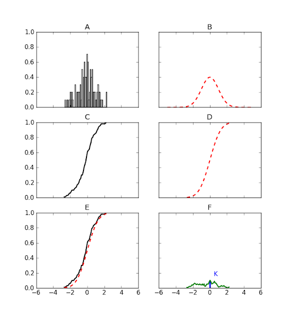
Today's problem is to determine if a sample of N numbers (Fig.A) is compatible with a given probability distribution (Fig.B). Instead of the probability distribution functions we will consider the two cumulative probability distributions (Fig.C and D). The Kolmogorov-Smirnov statistics, K, is the maximum distance from zero of the difference between the two cumulative distribution functions (Fig.E and F). In the ideal limit of infinite data points, the analytic expression for the probability distribtion of K is known and in the next post we will compute the p-value for the initial sample.


Useful Wikipedia links for further reading are:
Kolmogorov-Smirnov test
Donkster's theorem
Brownian bridge


This is the code I used to generate the figures:


import matplotlib.pyplot as plt
import numpy as np
from scipy.stats import norm
from scipy.stats import cumfreq


mean, sigma, nvariates = 0, 1, 100
np.random.seed(2)
sample = norm.rvs(mean, sigma, size=nvariates)


fig, axs = plt.subplots(nrows=3, ncols=2, sharex=True, sharey=True)


# Fig.A
ax = axs[0, 0]
ax.hist(sample, 50, normed=1, facecolor='white')
ax.set_title('A')


# Fig.B
ax = axs[0, 1]
x = np.arange(-5, 5, 0.001)
ax.plot(x, norm.pdf(x, mean, sigma), 'r--', linewidth=2)
ax.set_title('B')


# Fig.C
ax = axs[1, 0]
partialsums, xmin, xstep, extrapoints = cumfreq(sample, 50)
x = np.arange(xmin, xmin+50*xstep, xstep)
partialfractions = partialsums/nvariates
ax.plot(x, partialfractions, 'k', linewidth=2)
ax.set_title('C')


# Fig.D
ax = axs[1, 1]
ax.plot(x, norm.cdf(x, mean, sigma), 'r--', linewidth=2)
ax.set_title('D')


# Fig.E
ax = axs[2, 0]
ax.plot(x, partialfractions, 'k', linewidth=2)
ax.plot(x, norm.cdf(x, mean, sigma), 'r--', linewidth=2)
ax.set_title('E')


# Fig.F
ax = axs[2, 1]
differences = abs(partialfractions - norm.cdf(x, mean, sigma))
ax.plot(x, differences, color='g', linewidth=2)
xline = xmin+xstep*np.argmax(differences)
yline = np.amax(differences)
ax.vlines(xline, ymin=0, ymax=yline, color='b', linewidth=3)
ax.text(xline+0.5, 1.5*yline, 'K', color='b')
ax.set_title('F')


plt.show()


Addendum: the code above can be 
improved

2012-07-23

Random variables in Python


import matplotlib.pyplot as plt
import numpy as np
from scipy.stats import norm


# generate 1000 instances of a normal random variable
mean, sigma = 0, 1
sample = norm.rvs(mean, sigma, size=1000)


# a 50-bin histogram of the sample
plt.hist(sample, 50, normed=1, facecolor='white')


# the population distribution
range = np.arange(-5, 5, 0.001)
plt.plot(range, norm.pdf(range, mean, sigma), color='red', linewidth=4)


plt.show()

Result:


Addendum: the code above can be improved

2012-07-22

How to plot a normal distribution in Python


Python code (slightly adapted from StackOverflow) to plot a normal distribution.

# Plot a normal distribution


import numpy as np
import matplotlib.pyplot as plt
from scipy.stats import norm


mean = 0
standard_deviation = 1


# Plot between -10 and 10 with .001 steps.
range = np.arange(-10, 10, 0.001)


# Mean = 0, SD = 1.
plt.plot(range, norm.pdf(range, mean, standard_deviation))


plt.show()

Result:


Addendum: the code above can be 
improved